

本文主要基于以下参考:
[1] John T. Betts. Survey of Numerical Methods for Trajectory Optimization.
[2] Anil V. Rao. A Survey of Numerical Methods For Optimal Control.
[3] John T. Betts. Practical Methods for Optimal Control and Estimation Using Nonlinear Programming 2nd.
[4] A E. Bryson. Applied Optimal Control.
[5] KIRK. Optimal Control Theory: An Introduction.
[6] Matthew Kelly. An Introduction to Trajectory Optimization: How to Do Your Own Direct Collocation.
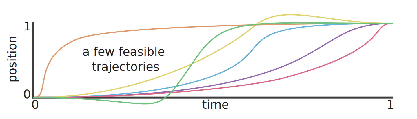
下面继续看[4] 2.7节,最优控制问题描述为:
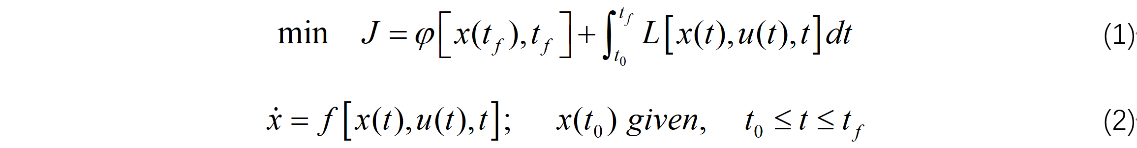
在前面的几节中,我们考虑的最优控制问题被限制为终端时间固定,终端约束形式不同,从本节开始,考虑终端时间可变的最优控制问题,本节之后可以对更多的最优控制问题进行求解。
类似于前面对约束的处理,同样可以得到:

与前面不同的是,这里我们还要考虑由于终端时间 tf 变化导致的增量:
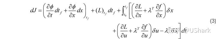
同样对上式中最后一部分分部积分并整理可以得到:

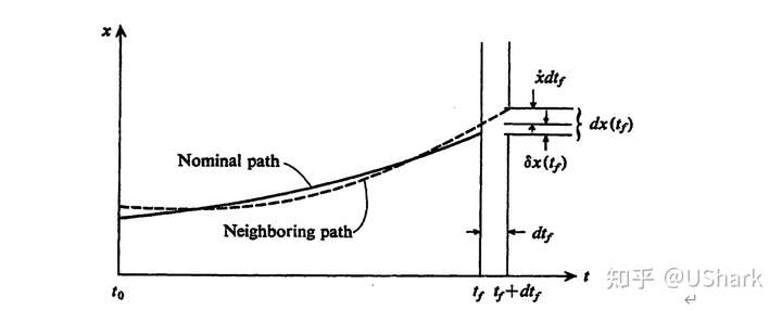
此时,变分 δx 表示时间固定,两条 x 曲线在时间 t 处的变分, dx 表示曲线在端点处的变化量可以写作:

因此由(5)式,可以得到

代入到式(4)中可以得到:
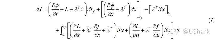
由于 δx(t0) 给定,以及 dtf , dx(tf) 的任意性可以得到:

在书中给出了很多相关的最优控制问题的例子。
下面给出一个具体的例子:
最优控制问题(Brachistochrone problem):

边界条件:

其中, g=9.8 。
同样类似地首先写出最优必要条件:

然后写出必要的边界条件:
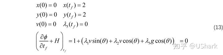
整理以上式子,形式比较复杂,注意到 L 和 f 均不含时间 t ,因此哈密顿函数在最优轨迹上为常数,且由(13)最后式可知 H=-1 ,因此可得:

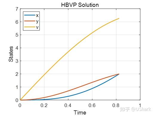
在对这个问题求解的过程中,由于时间自由,不好直接使用bvp来进行求解,因此将时间规范化到 [0,1] 区间内,然后将 tf 也当作边界条件来进行求解。
clear all;
g = 9.8;
% 初始化,时间区间为[0,1]
solinit = bvpinit(linspace(0,1),@BVPInit);
tol = 1E-10;
options = bvpset('RelTol',tol,'AbsTol',[tol tol tol tol tol tol tol],'Nmax', 5000);
sol = bvp4c(@BVPOde,@BVPbc,solinit,options);
time = sol.y(7)*sol.x; % get time
state = sol.y([1 2 3], :);
adjoint = sol.y([4 5 6],:);
control = atan(adjoint(1,:) .* state(3,:) ./ (adjoint(2,:).*state(3,:)+adjoint(3,:).*g));
mm.time= time;
mm.state = state;
mm.costate= adjoint;
mm.control = control;
figure(1); clf
plot(mm.time,mm.state,'LineWidth',2)
legend('x','y','v','Location','NorthWest')
grid on;
%axis([0 0.9 0 7])
title('HBVP Solution')
xlabel('Time');ylabel('States')
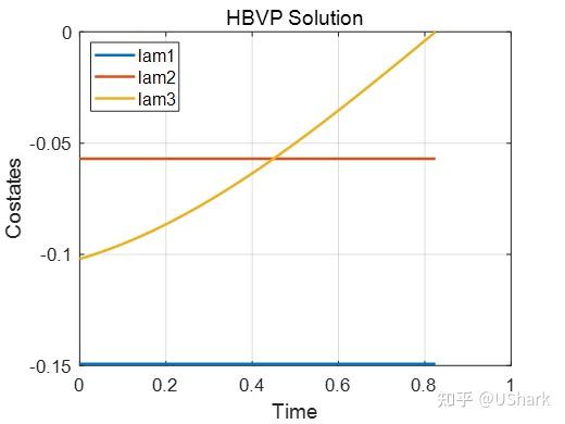
figure(2); clf
plot(mm.time,mm.costate,'LineWidth',2)
legend('lam1','lam2','lam3','Location','NorthWest')
grid on;
%axis([0 0.9 -0.5 0])
title('HBVP Solution')
xlabel('Time');ylabel('Costates')
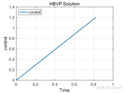
figure(3); clf
plot(mm.time,mm.control,'LineWidth',2)
legend('control','Location','NorthWest')
grid on;
%axis([0 0.9 -0.5 0])
title('HBVP Solution')
xlabel('Time');ylabel('control')%-------------------------------------------------------------------------?
function dydt=BVPOde(t, state)
g = 9.8;
x=state(1); y=state(2); v=state(3);
cx1=state(4); cx2=state(5); cx3=state(6);
tanth = cx1*v / (cx2*v+cx3*g);
th = atan(tanth);
sinth = sin(th);
costh = cos(th);
dydt=state(7)*[
v*sinth;
v*costh;
g*costh;
0;
0;
-(cx1*sinth+cx2*costh);
0];
end
%-------------------------------------------------------------------------function res=BVPbc(ya,yb)
g = 9.8;
x0=ya(1); y0=ya(2); v0=ya(3);
cx10=ya(4); cx20=ya(5); cx30=ya(6);
xf=yb(1); yf=yb(2); vf=yb(3);
cx1f=yb(4); cx2f=yb(5); cx3f=yb(6);
tanth = cx1f*vf / (cx2f*vf+cx3f*g);
th = atan(tanth);
sinth = sin(th);
costh = cos(th);
res = [x0;
y0;
v0;
xf-2;
yf-2;
cx3f;
1+cx1f*vf*sinth+cx2f*vf*costh+cx3f*g*costh];
end
%-------------------------------------------------------------------------?
更多的最优控制问题可以参考[4] 中的2.7节给出了更多的问题示例。


评论(0)
您还未登录,请登录后发表或查看评论