

本文作为自己阅读论文后的总结和思考,不涉及论文翻译和模型解读,适合大家阅读完论文后交流想法,关于论文翻译可以查看参考文献。论文地址:https://arxiv.org/abs/1711.11053
一. 全文总结
本文提出了一个一般概率多步时间序列回归的框架。具体来说,本文利用了seq2seq神经网络的表达性和时间性质(例如,递归和卷积结构),分位数回归的非参数性质和Direct Multi-Horizon Forecasting的效率。为提高序列网络的稳定性和性能,设计了一种新的训练方案——分支序列(forking-sequences)训练方案。文章表明,在现实生活中的大规模预测中,该方法既能适应时间和静态协变量,也能跨越多个相关系列、不断变化的季节性、未来计划的事件峰值和冷启动。
二. 研究方法
-
将序列网络(如rnn)或一维cnn与QR和Multi-Horizon预测相结合。
-
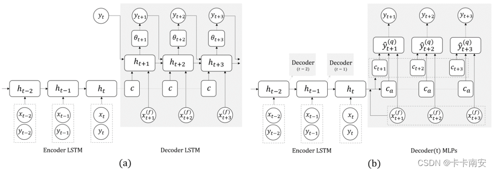
以MQRNN为例,Encoder为LSTM网络将所有历史编码为隐藏状态 ht。
-
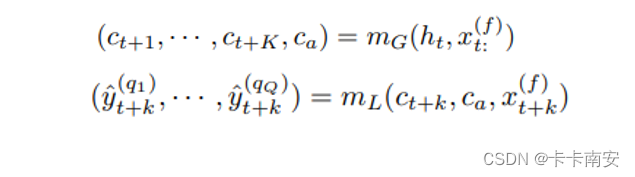
在Decoder部分设计了两个MLP分支,global MLP将编码器输出和所有未来输入汇总到两个信息中:针对 K 个未来点中的每一个一系列特定时段(horizon-specific)上下文 Ct+k,以及捕获公共信息的与时段无关(horizon-agnostic)的上下文 ca。local MLP适用于每个特定的时段。它结合了相应的未来输入和前面描述的全局 MLP 的两个上下文,然后输出该特定未来时间步长所需的所有分位数。
4.以最小化总分位数损失训练模型,在训练时采用分叉序列(forking-sequences)训练方案,即在训练时每一步都进行预测并计算损失函数。

5.优化Encoder的结构可以在一定程度上提升预测性能。
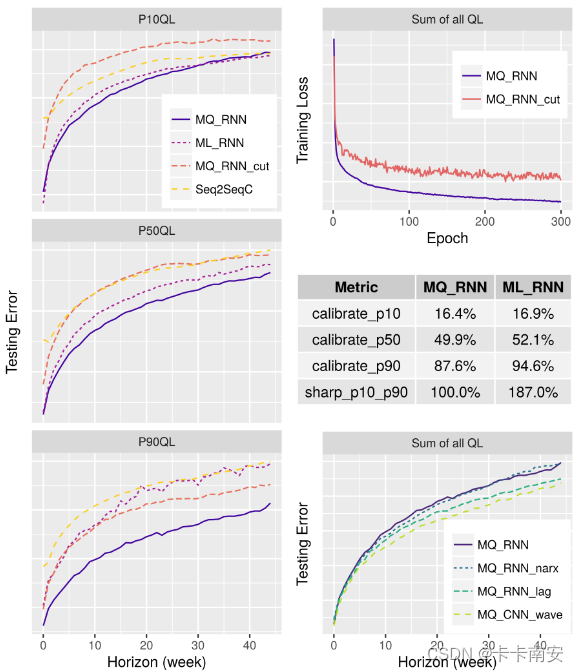
模型的预测性能如下图所示,比较了几个模型:
- MQ RNN:图 2b 中提出的模型,其他基准测试是它的变体,这意味着我们修改或剔除单个功能以模仿最先进的方法,同时尽最大努力控制所有其他设置/超参数。
- ML RNN:QL 更改为移位的对数高斯似然:log (y + 1) ∼ N (µ, σ2) 并预测 (ˆµ, ˆσ);
- MQ RNN cut:不使用分叉序列,而是通过 FCT 切割每个序列;切割在样本和epochs之间是随机的,以更好地利用数据中的所有信息;
- Seq2SeqC:将最先进的 Seq2Seq 结构与预测的 Log-Gaussian 参数相结合,并递归地使用一步超前估计均值作为后续预测的输入,通过教师强制和切割序列进行训练;值得注意的是,Seq2SeqC 是比 DeepAR 更通用和更有效的基准,因为它不限于相同的 LSTM 编码器/解码器,并且在估计边际多水平分布的情况下不需要重复的顺序采样。
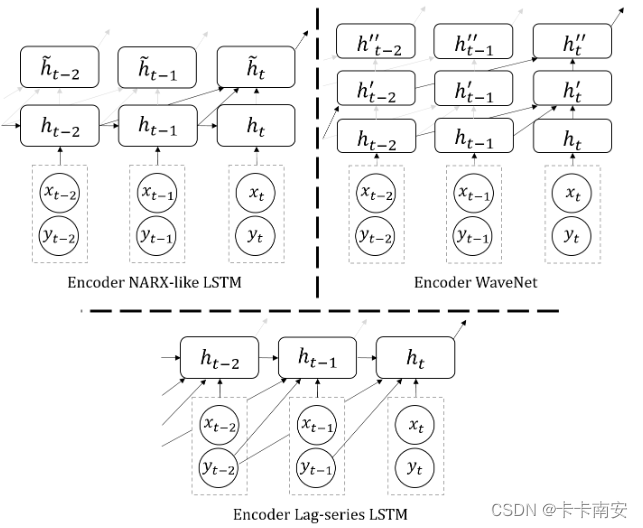
MQ-RNN 中的编码器可以进行替换,分别是具有最后 52 个状态的跳过连接的MQ-RNN narx , 具有最后 52 个需求值作为输入的MQ-RNN lag,带有扩张卷积层的 MQ CNN wave 。分位数估计为 q ∈ {0.1, 0.5, 0.9}(P10、P50 和 P90 预测)。
三. 结论
遥远的未来信息(例如假期)可以对近期的视野(预期)产生追溯影响,这就是global MLP 也使用未来信息的原因。
分叉序列(forking-sequences)使得每个任意长度的时间序列在我们的模型训练中充当单个样本,消除了数据增强的需要,并显著减少了训练时间。
MQRNN与MLRNN、Seq2Seq模型相比有更好的预测效果,将模型中的Encoder换成RNN_narx、RNN_lag及CNN_wave能提升预测效果。
四. 创新点
- 这是第一个将序列网络(如rnn)或一维cnn与QR和Multi-Horizon预测相结合的工作。MQ-RNN:其中总损失函数为单/多个分位数损失之和,输出为不同q值的所有分位数预测。
- 在预测时采用直接预测而非递归预测能有效避免误差累积。
- 提出了一种将序列神经网络与多视界预测相结合的高效训练方案,即forking-sequences,每个循环层对应一个具有相同权值的解码器(阴影框),在所有的时间点上进行训练并创建预测。
- 与DeepAR的不同之处在于使用了更实际的多视界策略(直接预测),这是一种更有效的训练策略,并直接生成准确的分位数。
五. 思考
在Encoder和Decoder上均可以做修改和创新,可与最新的时间序列预测模型结合,采用分位数回归的方法进行多视野预测。(这个forking-sequences我并不是特别理解是怎么实现的)
六. 参考文献
- 【时序】MQ-RNN 概率预测模型论文笔记
七. Pytorch实现
以下代码参考:https://github.com/jingw2/demand_forecast,修正了原代码中存在的一些错误,附添加了一些必要的注释让大家更好理解,代码中没有用到forking-sequences。
import torch
from torch import nn
import torch.nn.functional as F
from torch.optim import Adam

import numpy as np
import math
import os
import random
import matplotlib.pyplot as plt
import pickle
from tqdm import tqdm
import pandas as pd
from sklearn.preprocessing import StandardScaler, MinMaxScaler
from time import time
import argparse
from datetime import date
from progressbar import *
util(工具函数)
def get_data_path():
    folder = os.path.dirname(__file__)
    return os.path.join(folder, "data")

def RSE(ypred, ytrue):
    rse = np.sqrt(np.square(ypred - ytrue).sum()) / \
            np.sqrt(np.square(ytrue - ytrue.mean()).sum())
    return rse

def quantile_loss(ytrue, ypred, qs):
    '''
    Quantile loss version 2
    Args:
    ytrue (batch_size, output_horizon)
    ypred (batch_size, output_horizon, num_quantiles)
    '''
    L = np.zeros_like(ytrue)
    for i, q in enumerate(qs):
        yq = ypred[:, :, i]
        diff = yq - ytrue
        L += np.max(q * diff, (q - 1) * diff)
    return L.mean()

def SMAPE(ytrue, ypred):
    ytrue = np.array(ytrue).ravel()
    ypred = np.array(ypred).ravel() + 1e-4
    mean_y = (ytrue + ypred) / 2.
    return np.mean(np.abs((ytrue - ypred) \
        / mean_y))

def MAPE(ytrue, ypred):
    ytrue = np.array(ytrue).ravel() + 1e-4
    ypred = np.array(ypred).ravel()
    return np.mean(np.abs((ytrue - ypred) \
        / ytrue))

def train_test_split(X, y, train_ratio=0.7):
    '''
    - X (array like): shape (num_samples, num_periods, num_features)
    - y (array like): shape (num_samples, num_periods)
    '''
    num_ts, num_periods, num_features = X.shape
    train_periods = int(num_periods * train_ratio)
    random.seed(2)
    Xtr = X[:, :train_periods, :]
    ytr = y[:, :train_periods]
    Xte = X[:, train_periods:, :]
    yte = y[:, train_periods:]
    return Xtr, ytr, Xte, yte

class StandardScaler:

    def fit_transform(self, y):
        self.mean = np.mean(y)
        self.std = np.std(y) + 1e-4
        return (y - self.mean) / self.std

    def inverse_transform(self, y):
        return y * self.std + self.mean

    def transform(self, y):
        return (y - self.mean) / self.std

class MaxScaler:

    def fit_transform(self, y):
        self.max = np.max(y)
        return y / self.max

    def inverse_transform(self, y):
        return y * self.max

    def transform(self, y):
        return y / self.max


class MeanScaler:

    def fit_transform(self, y):
        self.mean = np.mean(y)
        return y / self.mean

    def inverse_transform(self, y):
        return y * self.mean

    def transform(self, y):
        return y / self.mean

class LogScaler:

    def fit_transform(self, y):
        return np.log1p(y)

    def inverse_transform(self, y):
        return np.expm1(y)

    def transform(self, y):
        return np.log1p(y)


def gaussian_likelihood_loss(z, mu, sigma):
    '''
    Gaussian Liklihood Loss
    Args:
    z (tensor): true observations, shape (num_ts, num_periods)
    mu (tensor): mean, shape (num_ts, num_periods)
    sigma (tensor): standard deviation, shape (num_ts, num_periods)
    likelihood:
    (2 pi sigma^2)^(-1/2) exp(-(z - mu)^2 / (2 sigma^2))
    log likelihood:
    -1/2 * (log (2 pi) + 2 * log (sigma)) - (z - mu)^2 / (2 sigma^2)
    '''
    negative_likelihood = torch.log(sigma + 1) + (z - mu) ** 2 / (2 * sigma ** 2) + 6
    return negative_likelihood.mean()

def negative_binomial_loss(ytrue, mu, alpha):
    '''
    Negative Binomial Sample
    Args:
    ytrue (array like)
    mu (array like)
    alpha (array like)
    maximuze log l_{nb} = log Gamma(z + 1/alpha) - log Gamma(z + 1) - log Gamma(1 / alpha)
                - 1 / alpha * log (1 + alpha * mu) + z * log (alpha * mu / (1 + alpha * mu))
    minimize loss = - log l_{nb}
    Note: torch.lgamma: log Gamma function
    '''
    batch_size, seq_len = ytrue.size()
    likelihood = torch.lgamma(ytrue + 1. / alpha) - torch.lgamma(ytrue + 1) - torch.lgamma(1. / alpha) \
        - 1. / alpha * torch.log(1 + alpha * mu) \
        + ytrue * torch.log(alpha * mu / (1 + alpha * mu))
    return - likelihood.mean()

def batch_generator(X, y, num_obs_to_train, seq_len, batch_size):
    '''
    Args:
    X (array like): shape (num_samples, train_periods, num_features)
    y (array like): shape (num_samples, train_periods)
    num_obs_to_train (int): 训练的历史窗口长度
    seq_len (int): sequence/encoder/decoder length
    batch_size (int)
    '''
    num_ts, num_periods, _ = X.shape
    if num_ts < batch_size:
        batch_size = num_ts
    t = random.choice(range(num_obs_to_train, num_periods-seq_len)) # 从num_obs_to_train和num_periods-seq_len-1之间随机选一个整数,作为预测点
    batch = random.sample(range(num_ts), batch_size) # 从num_ts条数据中随机选择batch_size条
    X_train_batch = X[batch, t-num_obs_to_train:t, :] # (batch_size, num_obs_to_train, num_features)
    y_train_batch = y[batch, t-num_obs_to_train:t] # (batch_size, num_obs_to_train)
    Xf = X[batch, t:t+seq_len, :] # (batch_size, seq_len, num_features)
    yf = y[batch, t:t+seq_len] # (batch_size, seq_len)
    return X_train_batch, y_train_batch, Xf, yf
Model
class Decoder(nn.Module):

    def __init__(
        self,
        input_size,
        output_horizon,
        encoder_hidden_size,
        decoder_hidden_size,
        output_size):
        super(Decoder, self).__init__()
        self.global_mlp = nn.Linear(output_horizon * (encoder_hidden_size + input_size), \
                (output_horizon+1) * decoder_hidden_size)
        self.local_mlp = nn.Linear(decoder_hidden_size * 2 + input_size, output_size)
        self.decoder_hidden_size = decoder_hidden_size

    def forward(self, ht, xf):
        '''
        Args:
        ht (tensor): (num_samples, hidden_size)
        xf (tensor): (num_samples, seq_len, num_features)
        '''
        num_ts, output_horizon, num_features = xf.size()
        num_ts, hidden_size = ht.size()
        ht = ht.unsqueeze(1) # (num_samples, 1, hidden_size)
        ht = ht.expand(num_ts, output_horizon, hidden_size) # (num_samples, seq_len, hidden_size)
        # inp = (xf + ht).view(batch_size, -1) # batch_size, hidden_size, output_horizon
        inp = torch.cat([xf, ht], dim=2).view(num_ts, -1) # (num_samples, seq_len*(hidden_size+num_features) )
        contexts = self.global_mlp(inp) # (num_samples, (seq_len+1) * decoder_hidden_size )
        contexts = contexts.view(num_ts, output_horizon+1, self.decoder_hidden_size) # (num_samples, seq_len+1, decoder_hidden_size)
        ca = contexts[:, -1, :].view(num_ts, -1) # (num_samples, decoder_hidden_size)
        C = contexts[:, :-1, :] # (num_samples, seq_len, decoder_hidden_size)
        C = F.relu(C)
        y = []
        for i in range(output_horizon):
            ci = C[:, i, :].view(num_ts, -1) # (num_samples, decoder_hidden_size)
            xfi = xf[:, i, :].view(num_ts, -1) # (num_samples, num_features)
            inp = torch.cat([xfi, ci, ca], dim=1) # (num_samples, num_features+decoder_hidden_size+decoder_hidden_size)
            out = self.local_mlp(inp) # (num_samples, num_quantiles)
            y.append(out.unsqueeze(1))# out.unsqueeze(1): (num_samples, 1, num_quantiles)
        y = torch.cat(y, dim=1) # (num_samples, seq_len, num_quantiles)
        return y
class MQRNN(nn.Module):

    def __init__(
        self,
        output_horizon,
        num_quantiles,
        input_size,
        embedding_size=10,
        encoder_hidden_size=64,
        encoder_n_layers=3,
        decoder_hidden_size=64
        ):
        '''
        Args:
        output_horizon (int): output horizons to output in prediction
        num_quantiles (int): number of quantiles interests, e.g. 0.25, 0.5, 0.75
        input_size (int): feature size
        embedding_size (int): embedding size
        encoder_hidden_size (int): hidden size in encoder
        encoder_n_layers (int): encoder number of layers
        decoder_hidden_size (int): hidden size in decoder
        '''
        super(MQRNN, self).__init__()
        self.output_horizon = output_horizon
        self.encoder_hidden_size = encoder_hidden_size
        self.input_embed = nn.Linear(1, embedding_size) # time series embedding
        self.encoder = nn.LSTM(input_size + embedding_size, encoder_hidden_size, \
                    encoder_n_layers, bias=True, batch_first=True)
        self.decoder = Decoder(input_size, output_horizon, encoder_hidden_size,\
                    decoder_hidden_size, num_quantiles)

    def forward(self, X, y, Xf):
        '''
        Args:
        X (tensor like): shape (num_samples, num_obs_to_train, num_features)
        y (tensor like): shape (num_samples, num_obs_to_train)
        Xf (tensor like): shape (num_samples, seq_len, num_features)
        '''
        if isinstance(X, type(np.empty(2))):
            X = torch.from_numpy(X).float()
            y = torch.from_numpy(y).float()
            Xf = torch.from_numpy(Xf).float()
        num_ts, num_periods, num_features = X.size()
        y = y.unsqueeze(2) # (num_samples, num_obs_to_train, 1)
        y = self.input_embed(y) # (num_samples, num_obs_to_train, embedding_size)
        x = torch.cat([X, y], dim=2) # (num_samples, num_obs_to_train, num_features+embedding_size)
        # x = x.unsqueeze(0) # batch, seq_len, embed + num_features
        _, (h, c) = self.encoder(x) # h size (num_layers, num_samples, hidden_size)
        ht = h[-1, :, :] # (num_samples, hidden_size)
        # global mlp
        ht = F.relu(ht)
        ypred = self.decoder(ht, Xf) # (num_samples, seq_len, num_quantiles)
        return ypred
Load Data
num_epoches = 100
step_per_epoch = 3 #在一个epoch中,从训练集中提取step_per_epoch次训练数据
lr = 1e-3
n_layers = 1
encoder_hidden_size = 50
decoder_hidden_size = 20
embedding_size = 10 #将上一时刻的真实值编码为embedding_size长度
seq_len = 60 #预测的未来窗口长度
num_obs_to_train = 168  #训练的历史窗口长度
show_plot = True
run_test = True
standard_scaler = True
log_scaler = False
mean_scaler = False
batch_size = 64

device=torch.device("cuda:0" if torch.cuda.is_available() else "cpu")
# 读取数据
data = pd.read_csv("LD_MT200_hour.csv", parse_dates=["date"])
data["year"] = data["date"].apply(lambda x: x.year)
data["day_of_week"] = data["date"].apply(lambda x: x.dayofweek)
data = data.loc[(data["date"].dt.date >= date(2014, 1, 1)) & (data["date"].dt.date <= date(2014, 3, 1))]
print(data.shape)
plt.figure(figsize=(16, 4))
plt.plot(data['MT_200'])
data.head()

# 数据预处理
features = ["hour", "day_of_week"]
# hours = pd.get_dummies(data["hour"])
# dows = pd.get_dummies(data["day_of_week"])
years = data["year"]
hours = data["hour"]
dows = data["day_of_week"]
# MT_200 = data["MT_200"]
# yscaler = StandardScaler()
# MT_200 = yscaler.fit_transform(MT_200)
X = np.c_[np.asarray(hours),np.asarray(dows)] #X:(len,features)
num_features = X.shape[1]
num_periods = len(data)
X = np.asarray(X).reshape((-1, num_periods, num_features))
y = np.asarray(data["MT_200"]).reshape((-1, num_periods))
print("X_shape=",X.shape) # (series_num,len,features_num)
print("y_shape=",y.shape) # (series_num,len)
# X = np.tile(X, (10, 1, 1))
# y = np.tile(y, (10, 1))

输出:
X_shape= (1, 1440, 2)
y_shape= (1, 1440)
# 滑动窗口
def sliding_window(DataSet, width, multi_vector = True): #DataSet has to be as an Array
    if multi_vector: #三维 (num_samples,length,features)
        num_samples,length,features = DataSet.shape
    else: #二维 (num_samples,length)
        DataSet = DataSet[:,:,np.newaxis] #(num_samples,length,1)
        num_samples,length,features = DataSet.shape

    x = DataSet[:,0:width,:] #(num_samples,width,features)
    x = x[np.newaxis,:,:,:] #(1,num_samples,width,features)
    for i in range(length - width):
        i += 1
        tmp = DataSet[:,i:i + width,:]#(num_samples,width,features)
        tmp = tmp[np.newaxis,:,:,:] #(1,num_samples,width,features)
        x = np.concatenate([x,tmp],0) #(i+1,num_samples,width,features)
    return x

width = num_obs_to_train + seq_len
X_data = sliding_window(X, width, multi_vector = True) #(len-width+1,num_samples,width,features)
Y_data = sliding_window(y, width, multi_vector = False) #(len-width+1,num_samples,width,1)
print("x的维度为:",X_data.shape)
print("y的维度为:",Y_data.shape)
# 取其中一类序列
i = 0
X_data = X_data[:,i,:,:]
Y_data = Y_data[:,i,:,0]
print("x的维度为:",X_data.shape)
print("y的维度为:",Y_data.shape)

输出:
x的维度为: (1213, 1, 228, 2)
y的维度为: (1213, 1, 228, 1)
x的维度为: (1213, 228, 2)
y的维度为: (1213, 228)
# SPLIT TRAIN TEST
from sklearn.model_selection import train_test_split

Xtr, Xte, ytr, yte = train_test_split(X_data, Y_data,
                                    test_size=0.3,
                                    random_state=0,
                                    shuffle=False)
print("X_train:{},y_train:{}".format(Xtr.shape,ytr.shape))
print("X_test:{},y_test:{}".format(Xte.shape,yte.shape))

输出:
X_train:(849, 228, 2),y_train:(849, 228)
X_test:(364, 228, 2),y_test:(364, 228)
# 标准化
yscaler = None
if standard_scaler:
    yscaler = StandardScaler()
elif log_scaler:
    yscaler = LogScaler()
elif mean_scaler:
    yscaler = MeanScaler()
if yscaler is not None:
    ytr = yscaler.fit_transform(ytr)
#构造Dtaloader
Xtr=torch.as_tensor(torch.from_numpy(Xtr), dtype=torch.float32)
ytr=torch.as_tensor(torch.from_numpy(ytr),dtype=torch.float32)
Xte=torch.as_tensor(torch.from_numpy(Xte), dtype=torch.float32)
yte=torch.as_tensor(torch.from_numpy(yte),dtype=torch.float32)

train_dataset=torch.utils.data.TensorDataset(Xtr,ytr) #训练集dataset
train_Loader=torch.utils.data.DataLoader(train_dataset,batch_size=batch_size)
Train
Args:
- X (array like): shape (num_samples, num_periods, num_features)
- y (array like): shape (num_samples, num_periods)
- epochs (int): number of epochs to run
- step_per_epoch (int): steps per epoch to run
- num_obs_to_train (int): The length of the history window for training
- seq_len (int): output horizon
- likelihood (str): what type of likelihood to use, default is gaussian
- num_skus_to_show (int): how many skus to show in test phase
- num_results_to_sample (int): how many samples in test phase as prediction
quantiles = [0.1,0.5,0.9]
# 定义模型和优化器
num_ts, num_periods, num_features = X.shape
num_quantiles = len(quantiles)
model = MQRNN(
seq_len,
num_quantiles,
num_features,
embedding_size,
encoder_hidden_size,
n_layers,
decoder_hidden_size
).to(device)
optimizer = Adam(model.parameters(), lr=lr)
random.seed(2)
losses = []
cnt = 0
# training
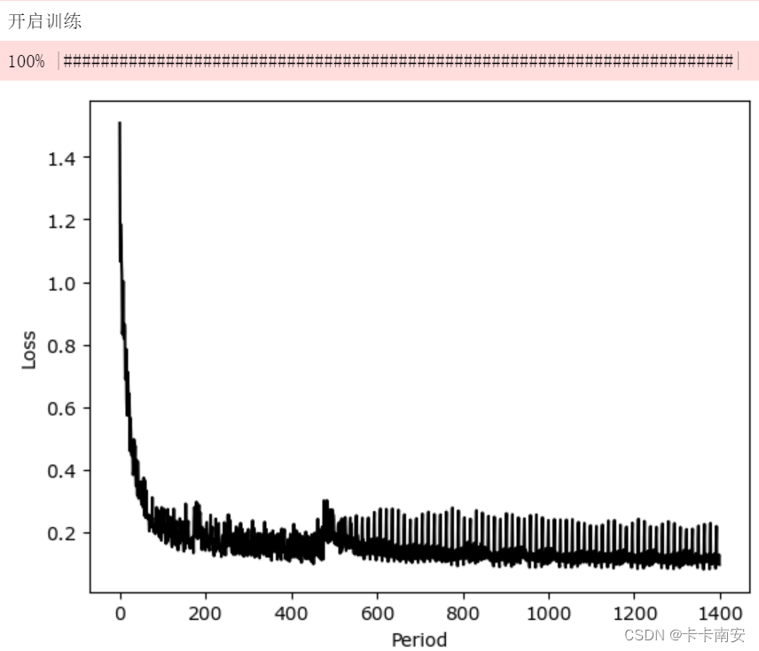
print("开启训练")
progress = ProgressBar()
for epoch in progress(range(num_epoches)):
# print("Epoch {} start...".format(epoch))
for x,y in train_Loader:
x = x.to(device) # (batch_size, num_obs_to_train+seq_len, num_features)
y = y.to(device) # (batch_size, num_obs_to_train+seq_len)
Xtrain = x[:,:num_obs_to_train,:].float() # (batch_size, num_obs_to_train, num_features)
ytrain = y[:,:num_obs_to_train].float() # (batch_size, num_obs_to_train)
Xf = x[:,-seq_len:,:].float() # (batch_size, seq_len, num_features)
yf = y[:,-seq_len:].float() # (batch_size, seq_len)
ypred = model(Xtrain, ytrain, Xf) # ypred:(batch_size, seq_len, num_quantiles)
# quantile loss
loss = torch.zeros_like(yf) #(batch_size, seq_len)
num_ts = Xf.size(0)
for q, rho in enumerate(quantiles):
ypred_rho = ypred[:, :, q].view(num_ts, -1) #(batch_size, seq_len)
# loss += (rho*torch.max(torch.zeros_like(yf),yf-ypred_rho) + (1-rho)*torch.max(torch.zeros_like(yf),ypred_rho-yf))
e = yf - ypred_rho
loss += torch.max(rho * e, (rho - 1) * e)
loss = loss.mean()
losses.append(loss.item())
optimizer.zero_grad()
loss.backward()
optimizer.step()
cnt += 1
if show_plot:
plt.plot(range(len(losses)), losses, "k-")
plt.xlabel("Period")
plt.ylabel("Loss")
plt.show()
Test
# test
print("开启测试")
X_test_sample = Xte[:,:,:].reshape(-1,num_obs_to_train+seq_len,num_features).to(device) # (num_samples, num_obs_to_train+seq_len, num_features)
y_test_sample = yte[:,:].reshape(-1,num_obs_to_train+seq_len).to(device) # (num_samples, num_obs_to_train+seq_len)

X_test = X_test_sample[:,:num_obs_to_train,:] # (num_samples, num_obs_to_train, num_features)
Xf_test = X_test_sample[:, -seq_len:, :] # (num_samples, seq_len, num_features)
y_test = y_test_sample[:, :num_obs_to_train] # (num_samples, num_obs_to_train)
yf_test = y_test_sample[:, -seq_len:] # (num_samples, seq_len)
if yscaler is not None:
    y_test = yscaler.transform(y_test)

ypred = model(X_test, y_test, Xf_test) # ypred:(num_samples, seq_len, num_quantiles)
ypred = ypred.cpu().detach().numpy()
if yscaler is not None:
    ypred = yscaler.inverse_transform(ypred)
ypred = np.maximum(0, ypred)

p50 = ypred[:,:,1] #(num_samples, seq_len)
p90 = ypred[:,:,2]
p10 = ypred[:,:,0]

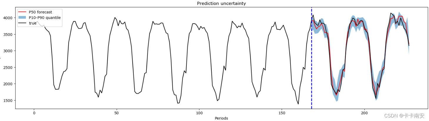
i = -1 #选取其中一条序列进行可视化
if show_plot: # 序列总长度为:历史窗口长度(num_obs_to_train)+预测长度(seq_len)
    plt.figure(1, figsize=(20, 5))
    plt.plot([k + seq_len + num_obs_to_train - seq_len for k in range(seq_len)], p50[i,:], "r-") # 绘制50%分位数曲线
    # 绘制10%-90%分位数阴影
    plt.fill_between(x=[k + seq_len + num_obs_to_train - seq_len for k in range(seq_len)], y1=p10[i,:], y2=p90[i,:], alpha=0.5)
    plt.title('Prediction uncertainty')
    yplot = y_test_sample[i,:].cpu() #真实值 (1, seq_len+num_obs_to_train)
    plt.plot(range(len(yplot)), yplot, "k-")
    plt.legend(["P50 forecast", "P10-P90 quantile", "true"], loc="upper left")
    ymin, ymax = plt.ylim()
    plt.vlines(seq_len + num_obs_to_train - seq_len, ymin, ymax, color="blue", linestyles="dashed", linewidth=2)
    plt.ylim(ymin, ymax)
    plt.xlabel("Periods")
    plt.ylabel("Y")
    plt.show()
#评价指标
pred_up  = p90[:,:].reshape(-1,seq_len) #(num_samples,seq_len)
pred_mid = p50[:,:].reshape(-1,seq_len) #(num_samples,seq_len)
pred_low = p10[:,:].reshape(-1,seq_len) #(num_samples,seq_len)
true = yf_test.cpu().detach().numpy()[:,:].reshape(-1,seq_len) #(num_samples,seq_len)
test_samples, seq_len = true.shape
u = 0.9-0.1

# 1. PICP(PI coverage probability) 要求大于等于区间分位数
PICP = 0
for i in range(test_samples):
    count = 0
    for j in range(seq_len):
        if true[i,j] > pred_low[i,j] and true[i,j] < pred_up[i,j]:
            count += 1
    picp = count / seq_len
    PICP += picp
PICP = PICP / test_samples
print("PICP:",PICP)

# 2. PINAW(PI normalized averaged width) 用于定义区间的狭窄程度,在保证准确性的前提下越小越好
PINAW = 0
for i in range(test_samples):
    width = 0
    true_max = np.max(true[i,:])
    true_min = np.min(true[i,:])
    for j in range(seq_len):
        width += (pred_up[i,j]-pred_low[i,j])
    width /= seq_len
    pinaw = (width / (true_max-true_min))
    PINAW += pinaw
PINAW = PINAW / test_samples
print("PINAW:",PINAW)

# 3. CWC(coverage width-based criterion) 综合考虑区间覆盖率和狭窄程度, 越小越好
g = 50 #取值在50-100
error = math.exp(-g * (PICP - u))
if PICP >= u:
    r = 0
else:
    r = 1
CWC = PINAW * (1 + r * error)
print("CWC:",CWC)

# 4. CRPS(continuous ranked probability score) 综合评价指标,量化一个连续概率分布(理论值)与确定性观测样本(真实值)间的差异,可视为平均绝对误差(MAE)在连续概率分布上的推广
# https://avoid.overfit.cn/post/302f7305a414449a9eb2cfa628d15853
def crps(y_true, y_pred, sample_weight=None):
    num_samples = y_pred.shape[0]
    absolute_error = np.mean(np.abs(y_pred - y_true), axis=0)
    if num_samples == 1:
        return np.average(absolute_error, weights=sample_weight)
    y_pred = np.sort(y_pred, axis=0) #(3,60)
    diff = y_pred[1:] - y_pred[:-1] #一阶差分
    weight = np.arange(1, num_samples) * np.arange(num_samples - 1, 0, -1)
    weight = np.expand_dims(weight, -1)
    per_obs_crps = absolute_error - np.sum(diff * weight, axis=0) / num_samples**2
    return np.average(per_obs_crps, weights=sample_weight)
CRPS = 0
for i in range(test_samples):
    y_pred = np.concatenate([pred_up[i,None,:],pred_mid[i,None,:],pred_low[i,None,:]],axis=0) #(3,60)
    y_true = true[i,:] #(1,60)
    c = crps(y_true,y_pred)
    CRPS += c
CRPS = CRPS / test_samples
print("CRPS:",CRPS)

# 5. P50 quantile MAE
MAE = 0
for i in range(test_samples):
    error = 0
    for j in range(seq_len):
        error += np.abs(true[i,j]-pred_mid[i,j])
    mae = error / seq_len
    MAE += mae
MAE = MAE / test_samples
print("P50 quantile MAE:",MAE)

# 6. # P50 quantile MAPE
MAPe = 0
for i in range(test_samples):
    mape = MAPE(true[i,:], pred_mid[i,:])
    MAPe += mape
MAPe = MAPe / test_samples
print("P50 quantile MAPE: {}".format(MAPe))

输出:
PICP: 0.8539377289377285
PINAW: 0.14504172429726733
CWC: 0.14504172429726733
CRPS: 81.07067743545147
P50 quantile MAE: 102.47593481601817
P50 quantile MAPE: 0.039683054390639724


评论(0)
您还未登录,请登录后发表或查看评论