

在一篇博客中,通过分析helloword的自动求导和节写求导简单例子,了解了Ceres的基本流程。本片博客在上一片基础之上,以高博十四讲内容为基础,分析Ceres两个使用案例
一、曲线拟合
1、问题描述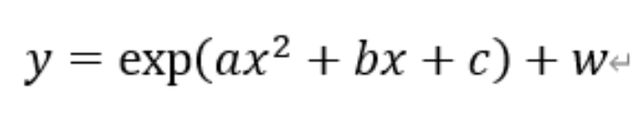
其中a,b,c为待估计的参数,w为噪声。在程序里利用模型生成x,y的数据,在给数据添加服从高斯分布的噪声。之后用ceres优化求解参数a,b,c。
2、求解代码
代码部分仍然与上一篇博客类似,分为三个部分
(1)、第一部分:构建cost fuction,即代价函数
struct CURVE_FITTING_COST {
  CURVE_FITTING_COST(double x, double y) : _x(x), _y(y) {}

  // 残差的计算
  template<typename T>
  // 模型参数,有3维
  bool operator()(const T *const abc, T *residual) const {
    residual[0] = T(_y) - ceres::exp(abc[0] * T(_x) * T(_x) + abc[1] * T(_x) + abc[2]); // y-exp(ax^2+bx+c)
    return true;
  }
  const double _x, _y;    // x,y数据
};
template
template<typename T>简单用法_realjc的博客-CSDN博客_template
利用operator()使得该结构体成为一个拟函数。这种方法定义使得Ceres可以像调用函数一样对该结构体的对象进行调用例如(对象为a)a
(2)第二部分:通过代价函数构建待求解的优化问题
// 构建最小二乘问题
  ceres::Problem problem;
  for (int i = 0; i < N; i++) {
    problem.AddResidualBlock(     // 向问题中添加误差项
      // 使用自动求导,模板参数:误差类型,输出维度,输入维度,维数要与前面struct中一致
      new ceres::AutoDiffCostFunction<CURVE_FITTING_COST, 1, 3>
      (new CURVE_FITTING_COST(x_data[i], y_data[i])),
      nullptr,            // 核函数,这里不使用,为空
      abc                 // 待估计参数
    );
}

残差函数维度为1,参数维度为3。
(3)、 第三部分:配置求解器参数并求解问题
// 配置求解器
  ceres::Solver::Options options;     // 这里有很多配置项可以填
  options.linear_solver_type = ceres::DENSE_NORMAL_CHOLESKY;  // 增量方程如何求解
  options.minimizer_progress_to_stdout = true;   // 输出到cout

  ceres::Solver::Summary summary;                // 优化信息
  chrono::steady_clock::time_point t1 = chrono::steady_clock::now();
  ceres::Solve(options, &problem, &summary);  // 开始优化
调用Solve函数进行求解,可以在options中配置。例如,可以选择使用Line Search或者Trust Region 迭代次数,步长等等
(4)完整代码
#include <iostream>
#include <opencv2/core/core.hpp>
#include <ceres/ceres.h>
#include <chrono>

using namespace std;

// 代价函数的计算模型
struct CURVE_FITTING_COST {
  CURVE_FITTING_COST(double x, double y) : _x(x), _y(y) {}

  // 残差的计算
  template<typename T>
  // 模型参数,有3维
  bool operator()(const T *const abc, T *residual) const {
    residual[0] = T(_y) - ceres::exp(abc[0] * T(_x) * T(_x) + abc[1] * T(_x) + abc[2]); // y-exp(ax^2+bx+c)
    return true;
  }

  const double _x, _y;    // x,y数据
};

int main(int argc, char **argv) {
  double ar = 1.0, br = 2.0, cr = 1.0;         // 真实参数值
  double ae = 2.0, be = -1.0, ce = 5.0;        // 估计参数值
  int N = 100;                                 // 数据点
  double w_sigma = 1.0;                        // 噪声Sigma值
  double inv_sigma = 1.0 / w_sigma;
  cv::RNG rng;                                 // OpenCV随机数产生器

  vector<double> x_data, y_data;      // 数据
  for (int i = 0; i < N; i++) {
    double x = i / 100.0;
    x_data.push_back(x);
    y_data.push_back(exp(ar * x * x + br * x + cr) + rng.gaussian(w_sigma * w_sigma));
  }

  double abc[3] = {ae, be, ce};

  // 构建最小二乘问题
  ceres::Problem problem;
  for (int i = 0; i < N; i++) {
    problem.AddResidualBlock(     // 向问题中添加误差项
      // 使用自动求导,模板参数:误差类型,输出维度,输入维度,维数要与前面struct中一致
      new ceres::AutoDiffCostFunction<CURVE_FITTING_COST, 1, 3>
      (new CURVE_FITTING_COST(x_data[i], y_data[i])),
      nullptr,            // 核函数,这里不使用,为空
      abc                 // 待估计参数
    );
  }

  // 配置求解器
  ceres::Solver::Options options;     // 这里有很多配置项可以填
  options.linear_solver_type = ceres::DENSE_NORMAL_CHOLESKY;  // 增量方程如何求解
  options.minimizer_progress_to_stdout = true;   // 输出到cout

  ceres::Solver::Summary summary;                // 优化信息
  chrono::steady_clock::time_point t1 = chrono::steady_clock::now();
  ceres::Solve(options, &problem, &summary);  // 开始优化
  chrono::steady_clock::time_point t2 = chrono::steady_clock::now();
  chrono::duration<double> time_used = chrono::duration_cast<chrono::duration<double>>(t2 - t1);
  cout << "solve time cost = " << time_used.count() << " seconds. " << endl;

  // 输出结果
  cout << summary.BriefReport() << endl;
  cout << "estimated a,b,c = ";
  for (auto a:abc) cout << a << " ";
  cout << endl;

  return 0;
}
(5)运行结果
iter      cost      cost_change  |gradient|   |step|    tr_ratio  tr_radius  ls_iter  iter_time  total_time
   0  1.597873e+06    0.00e+00    3.52e+06   0.00e+00   0.00e+00  1.00e+04        0    6.16e-04    6.42e-04
   1  1.884440e+05    1.41e+06    4.86e+05   9.88e-01   8.82e-01  1.81e+04        1    6.79e-04    1.35e-03
   2  1.784821e+04    1.71e+05    6.78e+04   9.89e-01   9.06e-01  3.87e+04        1    6.78e-04    2.03e-03
   3  1.099631e+03    1.67e+04    8.58e+03   1.10e+00   9.41e-01  1.16e+05        1    6.14e-04    2.66e-03
   4  8.784938e+01    1.01e+03    6.53e+02   1.51e+00   9.67e-01  3.48e+05        1    6.14e-04    3.28e-03
   5  5.141230e+01    3.64e+01    2.72e+01   1.13e+00   9.90e-01  1.05e+06        1    6.59e-04    3.94e-03
   6  5.096862e+01    4.44e-01    4.27e-01   1.89e-01   9.98e-01  3.14e+06        1    6.16e-04    4.56e-03
   7  5.096851e+01    1.10e-04    9.53e-04   2.84e-03   9.99e-01  9.41e+06        1    6.54e-04    5.22e-03
solve time cost = 0.00536211 seconds.
Ceres Solver Report: Iterations: 8, Initial cost: 1.597873e+06, Final cost: 5.096851e+01, Termination: CONVERGENCE
estimated a,b,c = 0.890908 2.1719 0.943628
二、Ceres求解BA
BA(捆绑调整,也叫光束平差法)将相机位姿和空间特征点放在一起同时优化。本文重点介绍Ceres的使用,BA以及残差函数构建参见下面非常好的博客。
Bundle Adjustment简述_记起来就随便写写-CSDN博客
这部分内容仍然是分为三个部分进行介绍,第二与第三部分与上面例子类似,残差函数稍有不同。
第一二部分:残差函数
class SnavelyReprojectionError {
public:
    //传入的是观测值(x,y两个方向)
    SnavelyReprojectionError(double observation_x, double observation_y) : observed_x(observation_x), observed_y(observation_y) {}
    template<typename T>
    bool operator()(const T *const camera,
                    const T *const point,
                    T *residuals) const {
        // camera[0,1,2] are the angle-axis rotation
        T predictions[2];
        CamProjectionWithDistortion(camera, point, predictions);
        residuals[0] = predictions[0] - T(observed_x);
        residuals[1] = predictions[1] - T(observed_y);

        return true;
    }

    // camera : 9 dims array
    // [0-2] : angle-axis rotation
    // [3-5] : translateion
    // [6-8] : camera parameter, [6] focal length, [7-8] second and forth order radial distortion
    // point : 3D location.
    // predictions : 2D predictions with center of the image plane.
    template<typename T>
    static inline bool CamProjectionWithDistortion(const T *camera, const T *point, T *predictions) {
        // Rodrigues' formula
        T p[3];
        AngleAxisRotatePoint(camera, point, p);
        // camera[3,4,5] are the translation
        p[0] += camera[3];
        p[1] += camera[4];
        p[2] += camera[5];
        // Compute the center for distortion
        T xp = -p[0] / p[2];
        T yp = -p[1] / p[2];
        // Apply second and fourth order radial distortion
        const T &l1 = camera[7];
        const T &l2 = camera[8];
        T r2 = xp * xp + yp * yp;
        T distortion = T(1.0) + r2 * (l1 + l2 * r2);
        const T &focal = camera[6];
        predictions[0] = focal * distortion * xp;
        predictions[1] = focal * distortion * yp;
        return true;
    }
    static ceres::CostFunction *Create(const double observed_x, const double observed_y) {
        return (new ceres::AutoDiffCostFunction<SnavelyReprojectionError, 2, 9, 3>(
            new SnavelyReprojectionError(observed_x, observed_y)));
    }
private:
    double observed_x;
    double observed_y;
};
优化参数有两个,一个是相机参数包括9个分别是:平移3个,旋转3个一个焦距,两个镜头畸变系数,一个是空间三维点(x,y,z)。
残差函数也是2维的包括x,y两个方向。
残差函数详解
AngleAxisRotatePoint(camera, point, p);
该函数将世界坐标系投影到向极坐标系![]()
T xp = -p[0] / p[2];
T yp = -p[1] / p[2];
归一化到Z等于1的平面![]()
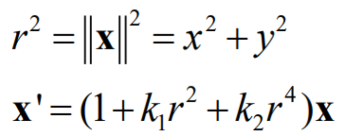
// Apply second and fourth order radial distortion
const T &k1 = camera[7];
const T &k2 = camera[8];

T r2 = xp * xp + yp * yp;
T distortion = T(1.0) +  (k1*r2 + k2 * r2*r2);
处理畸变问题
const T &focal = camera[6];
predictions[0] = focal * distortion * xp;
predictions[1] = focal * distortion * yp;
切换到像素坐标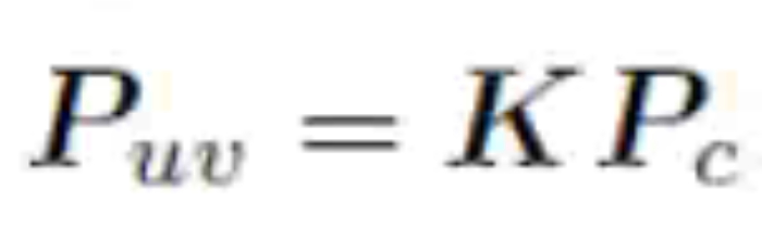
其中K即为相机的内参数,在本例中仅有焦距一个参数。
第二部分:构建待求解的优化问题
d SolveBA(BALProblem &bal_problem) {
    const int point_block_size = bal_problem.point_block_size();
    const int camera_block_size = bal_problem.camera_block_size();
    double *points = bal_problem.mutable_points();
    double *cameras = bal_problem.mutable_cameras();

    // Observations is 2 * num_observations long array observations
    // [u_1, u_2, ... u_n], where each u_i is two dimensional, the x
    // and y position of the observation.
    const double *observations = bal_problem.observations();
    ceres::Problem problem;

    for (int i = 0; i < bal_problem.num_observations(); ++i) {
        ceres::CostFunction *cost_function;

        // Each Residual block takes a point and a camera as input
        // and outputs a 2 dimensional Residual
        cost_function = SnavelyReprojectionError::Create(observations[2 * i + 0], observations[2 * i + 1]);

        // If enabled use Huber's loss function.
        ceres::LossFunction *loss_function = new ceres::HuberLoss(1.0);
        // Each observation corresponds to a pair of a camera and a point
        // which are identified by camera_index()[i] and point_index()[i]
        // respectively.
        double *camera = cameras + camera_block_size * bal_problem.camera_index()[i];
        double *point = points + point_block_size * bal_problem.point_index()[i];
        problem.AddResidualBlock(cost_function, loss_function, camera, point);
    }
第三部分: 配置求解器参数并求解问题
ceres::Solver::Options options;
options.linear_solver_type = ceres::LinearSolverType::SPARSE_SCHUR;
options.minimizer_progress_to_stdout = true;
ceres::Solver::Summary summary;
ceres::Solve(options, &problem, &summary);
std::cout << summary.FullReport() << "\n";
")


评论(0)
您还未登录,请登录后发表或查看评论